The CaDrA package currently provides four scoring functions to search for subsets of genomic features that are likely associated with a specific outcome of interest (e.g., protein expression, pathway activity, etc.)
- Kolmogorov-Smirnov Method (
ks) - Conditional Mutual Information Method (
revealer) - Wilcoxon Rank-Sum Method (
wilcox) - Custom - An User’s Provided Scoring Function
(
custom)
Below, we run candidate_search() over the top 3 starting
features using each of the four scoring functions described above.
Important Note:
- The legacy function
topn_eval()is equivalent to the recommendedcandidate_search()function
Load required datasets
- A
binary features matrixalso known asFeature Set(such as somatic mutations, copy number alterations, chromosomal translocations, etc.) The 1/0 row vectors indicate the presence/absence of ‘omics’ features in the samples. TheFeature Setmust be an object of class SummarizedExperiment from SummarizedExperiment package) - A vector of continuous scores (or
input_score) representing a functional response of interest (such as protein expression, pathway activity, etc.)
Kolmogorov-Smirnov scoring method
See ?ks_rowscore for more details
ks_topn_l <- CaDrA::candidate_search(
  FS = sim_FS,
  input_score = sim_Scores,
  method = "ks_pval",          # Use Kolmogorow-Smirnow scoring function
  weight = NULL,               # If weight is provided, perform a weighted-KS test
  alternative = "less",        # Use one-sided hypothesis testing
  search_method = "both",      # Apply both forward and backward search
  top_N = 3,                   # Evaluate top 3 starting points for the search
  max_size = 7,                # Allow at most 7 features in meta-feature matrix
  do_plot = FALSE,             # We will plot it AFTER finding the best hits
  best_score_only = FALSE      # Return meta-feature, its observed input scores and corresponding best score
)

# Now we can fetch the feature set of top N features that corresponded to the best scores over the top N search
ks_topn_best_meta <- topn_best(ks_topn_l)

# Visualize best meta-feature result
meta_plot(topn_best_list = ks_topn_best_meta)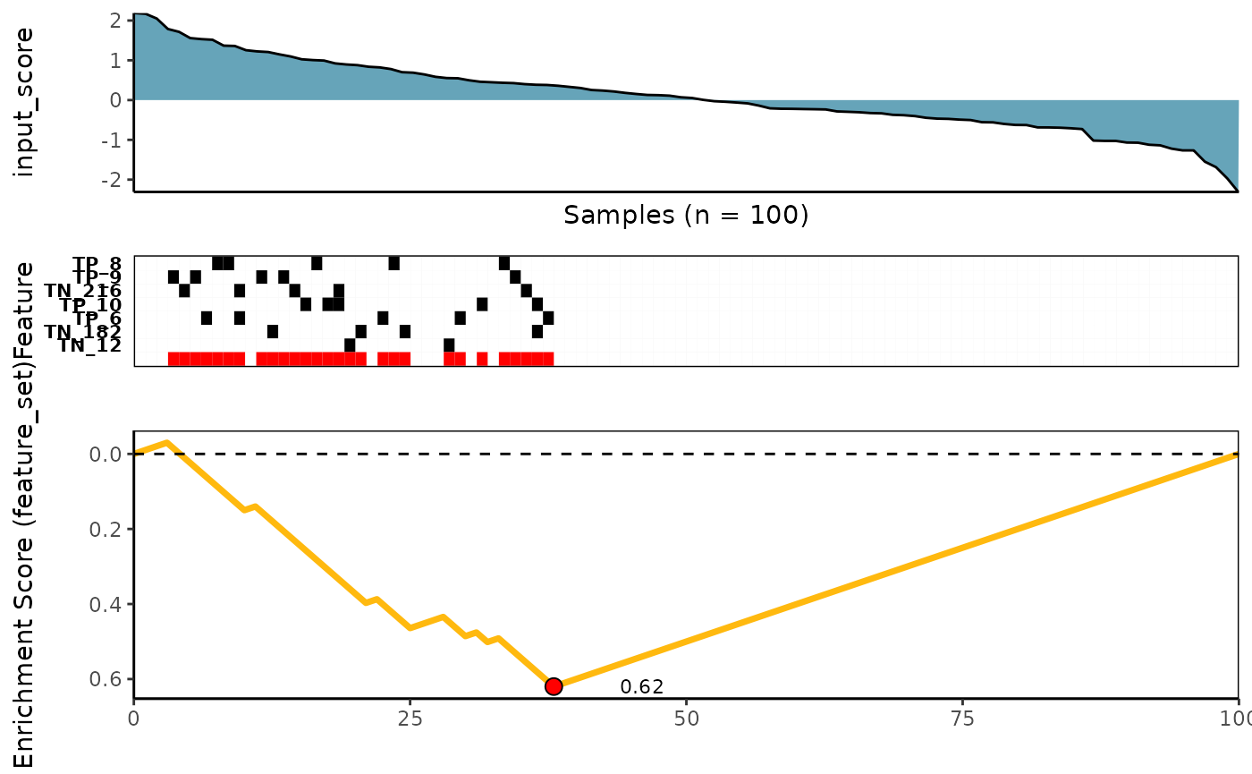
Wilcoxon Rank-Sum scoring method
See ?wilcox_rowscore for more details
wilcox_topn_l <- CaDrA::candidate_search(
  FS = sim_FS,
  input_score = sim_Scores,
  method = "wilcox_pval",      # Use Wilcoxon Rank-Sum scoring function
  alternative = "less",        # Use one-sided hypothesis testing
  search_method = "both",      # Apply both forward and backward search
  top_N = 3,                   # Evaluate top 3 starting points for the search
  max_size = 7,                # Allow at most 7 features in meta-feature matrix
  do_plot = FALSE,             # We will plot it AFTER finding the best hits
  best_score_only = FALSE      # Return meta-feature, its observed input scores and corresponding best score
)

# Now we can fetch the feature set of top N feature that corresponded to the best scores over the top N search
wilcox_topn_best_meta <- topn_best(topn_list = wilcox_topn_l)

# Visualize best meta-feature result
meta_plot(topn_best_list = wilcox_topn_best_meta)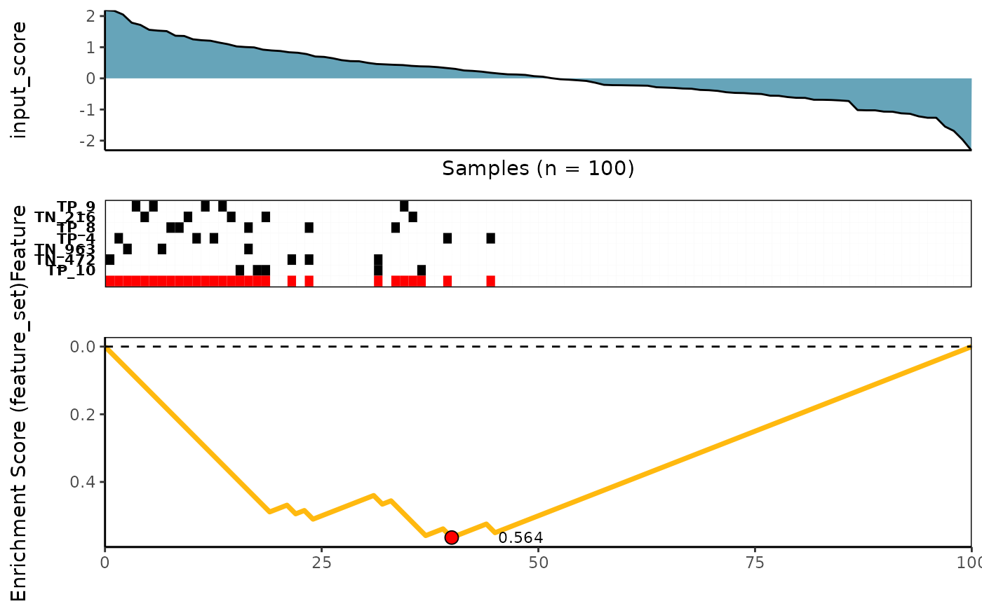
Conditional Mutual Information scoring method
See ?revealer_rowscore for more details
revealer_topn_l <- CaDrA::candidate_search(
  FS = sim_FS,
  input_score = sim_Scores,
  method = "revealer",         # Use REVEALER's CMI scoring function
  search_method = "both",      # Apply both forward and backward search
  top_N = 3,                   # Evaluate top 3 starting points for the search
  max_size = 7,                # Allow at most 7 features in meta-feature matrix
  do_plot = FALSE,             # We will plot it AFTER finding the best hits
  best_score_only = FALSE      # Return meta-feature, its observed input scores and corresponding best score
)

# Now we can fetch the ESet of top feature that corresponded to the best scores over the top N search
revealer_topn_best_meta <- topn_best(topn_list = revealer_topn_l)

# Visualize best meta-feature result
meta_plot(topn_best_list = revealer_topn_best_meta)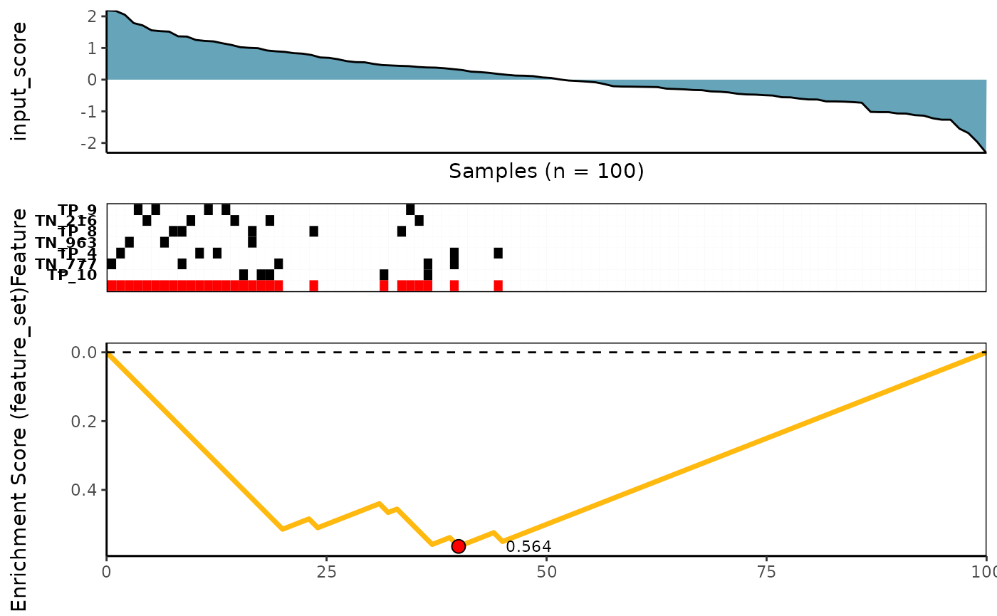
Custom - An user’s provided scoring method
See ?custom_rowscore for more details
# A customized function using ks-test function
customized_rowscore <- function(FS_mat, input_score, alternative){

  ks <- apply(FS_mat, 1, function(r){
    x = input_score[which(r==1)];
    y = input_score[which(r==0)];
    res <- ks.test(x, y, alternative=alternative)
    return(c(res$statistic, res$p.value))
  })

   # Obtain score statistics and p-values from KS method
  stat <- ks[1,]
  pval <- ks[2,]

  # Compute the -log scores for pval
  scores <- -log(pval)
  names(scores) <- rownames(FS_mat)

  # Re-order FS in a decreasing order (from most to least significant)
  # This comes in handy when doing the top-N evaluation of
  # the top N 'best' features
  scores <- scores[order(scores, decreasing=TRUE)]

  return(scores)

}

# Search for best features using a custom-defined function
custom_topn_l <- CaDrA::candidate_search(
  FS = sim_FS,
  input_score = sim_Scores,
  method = "custom",                                # Use custom scoring function
  custom_function = customized_rowscore,            # Use a customized scoring function
  custom_parameters = list(alternative = "less"),   # Additional parameters to pass to custom_function
  search_method = "both",                           # Apply both forward and backward search
  top_N = 3,                                        # Evaluate top 3 starting points for the search
  max_size = 7,                                     # Allow at most 7 features in meta-feature matrix
  do_plot = FALSE,                                  # We will plot it AFTER finding the best hits
  best_score_only = FALSE                           # Return meta-feature, its observed input scores and corresponding best score
)

# Now we can fetch the feature set of top N feature that corresponded to the best scores over the top N search
custom_topn_best_meta <- topn_best(topn_list = custom_topn_l)

# Visualize best meta-feature result
meta_plot(topn_best_list = custom_topn_best_meta)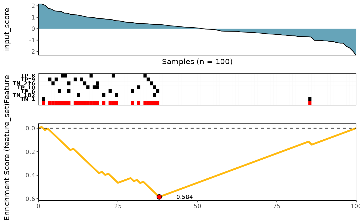
SessionInfo
sessionInfo()
R version 4.2.3 (2023-03-15)
Platform: x86_64-pc-linux-gnu (64-bit)
Running under: Ubuntu 22.04.2 LTS

Matrix products: default
BLAS:   /usr/lib/x86_64-linux-gnu/openblas-pthread/libblas.so.3
LAPACK: /usr/lib/x86_64-linux-gnu/openblas-pthread/libopenblasp-r0.3.20.so

locale:
 [1] LC_CTYPE=C.UTF-8       LC_NUMERIC=C           LC_TIME=C.UTF-8
 [4] LC_COLLATE=C.UTF-8     LC_MONETARY=C.UTF-8    LC_MESSAGES=C.UTF-8
 [7] LC_PAPER=C.UTF-8       LC_NAME=C              LC_ADDRESS=C
[10] LC_TELEPHONE=C         LC_MEASUREMENT=C.UTF-8 LC_IDENTIFICATION=C

attached base packages:
[1] stats4    stats     graphics  grDevices utils     datasets  methods
[8] base

other attached packages:
 [1] CaDrA_0.99.2                SummarizedExperiment_1.28.0
 [3] Biobase_2.58.0              GenomicRanges_1.50.2
 [5] GenomeInfoDb_1.34.9         IRanges_2.32.0
 [7] S4Vectors_0.36.2            BiocGenerics_0.44.0
 [9] MatrixGenerics_1.10.0       matrixStats_0.63.0
[11] BiocStyle_2.26.0

loaded via a namespace (and not attached):
 [1] sass_0.4.5             jsonlite_1.8.4         foreach_1.5.2
 [4] R.utils_2.12.2         gtools_3.9.4           bslib_0.4.2
 [7] highr_0.10             BiocManager_1.30.20    GenomeInfoDbData_1.2.9
[10] yaml_2.3.7             pillar_1.8.1           lattice_0.20-45
[13] glue_1.6.2             digest_0.6.31          XVector_0.38.0
[16] colorspace_2.1-0       htmltools_0.5.4        Matrix_1.5-3
[19] R.oo_1.25.0            plyr_1.8.8             pkgconfig_2.0.3
[22] misc3d_0.9-1           bookdown_0.33          zlibbioc_1.44.0
[25] purrr_1.0.1            scales_1.2.1           tibble_3.2.0
[28] farver_2.1.1           ggplot2_3.4.1          withr_2.5.0
[31] cachem_1.0.7           ppcor_1.1              cli_3.6.0
[34] magrittr_2.0.3         memoise_2.0.1          evaluate_0.20
[37] R.methodsS3_1.8.2      fs_1.6.1               fansi_1.0.4
[40] R.cache_0.16.0         doParallel_1.0.17      MASS_7.3-58.2
[43] gplots_3.1.3           textshaping_0.3.6      tools_4.2.3
[46] lifecycle_1.0.3        stringr_1.5.0          munsell_0.5.0
[49] DelayedArray_0.24.0    compiler_4.2.3         pkgdown_2.0.7
[52] jquerylib_0.1.4        caTools_1.18.2         systemfonts_1.0.4
[55] rlang_1.1.0            grid_4.2.3             RCurl_1.98-1.10
[58] iterators_1.0.14       labeling_0.4.2         bitops_1.0-7
[61] tcltk_4.2.3            rmarkdown_2.20         gtable_0.3.1
[64] codetools_0.2-19       reshape2_1.4.4         R6_2.5.1
[67] knitr_1.42             fastmap_1.1.1          utf8_1.2.3
[70] rprojroot_2.0.3        ragg_1.2.5             KernSmooth_2.23-20
[73] desc_1.4.2             stringi_1.7.12         parallel_4.2.3
[76] Rcpp_1.0.10            vctrs_0.6.0            xfun_0.37